By John Nardini
Click here for the PDF version
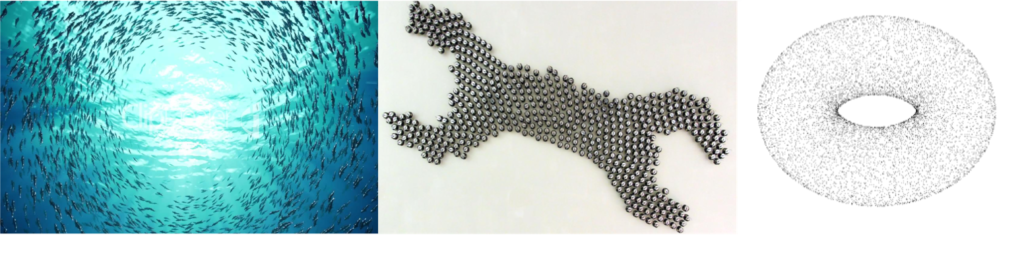
We may often observe that distinct shapes and structure emerge from the locations of individuals or discrete data samples. Topological data analysis (TDA) aims to summarize these patterns using concepts from algebraic topology and computational geometry. In this blog post, we will focus on the ideas and implementation of persistent homology, which is the most commonly used form of TDA.
Homology
To discuss persistent homology, we must first understand homology, which summarizes the shape of topological objects. An object’s homology is often summarized through the Betti numbers, which count the number of \(k\)-dimensional holes in the object. For example, the zeroth Betti number, \(\beta_0\), counts the number of connected components in an object, the first Betti number, \(\beta_1\), counts the number of loops, the second Betti number, \(\beta_2\), counts the number of trapped volumes, etc.
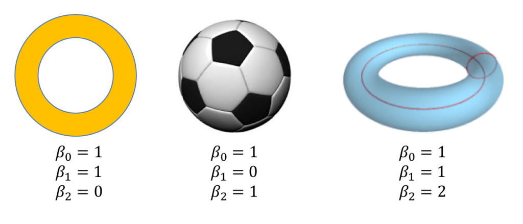
The Betti numbers for three topological objects are provided in Figure 2. A two-dimensional circle has one connected component, one loop, and no trapped volumes. The surface of a soccer ball has one connected component, no loops, and one trapped volume. To understand why there are no loops on the soccer ball, imagine tying a taught rubber band around it’s surface. If you moved the rubber band along the surface (while keeping it taught), the rubber band will eventually fall off, so there is no loop. The surface of a torus has one connected component, two loops, and one trapped area. There are two loops on the torus because if you placed a rubber band along either of the red curves in Figure 2, you would not be able to remove the rubber band without tearing it.
Simplicial complexes
The homology of the following collection of data points is simple — \(\beta_0\) is equal to the number of data points and all other Betti numbers are zero!

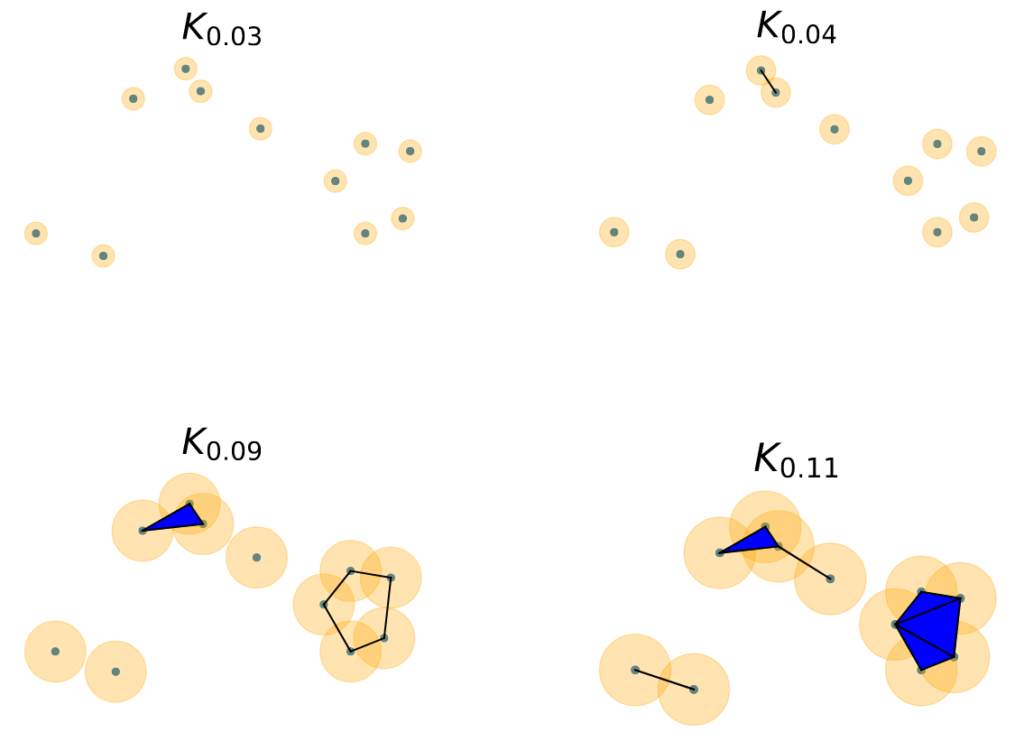
However, we may believe that there is an underlying structure to these discrete data points. To model this structure, we construct a simplicial complex, or collection of simple shapes that connect the data points together. We include each data point in our simplicial complex. We then choose a threshold distance, \(\epsilon\), and include the line connecting any two data points that are within \(\epsilon\) of each other to the simplicial complex, as shown in Figure 4. Additionally, we will place a triangle connecting any three data points that are all within \(\epsilon\) of each other. We could go on further (for example, by placing a tetrahedron between any four points that are each pairwise within \(\epsilon\) of each other), but we’ll stop here. Note that we have described how to create the Vietoris-Rips complex in this example, though there are other ways to construct simplicial complexes. For the chosen value of \(\epsilon\) in Figure 4, we notice that the simplicial complex’s Betti numbers are \(\beta_0=3,\beta_1=1,\beta_2=0\), etc.
Persistent Homology
In the previous section, we computed the homology of the data by constructing a simplicial complex, \(K_\epsilon\), by connecting points that are pairwise within \(\epsilon\) of each other. In Persistent homology, we consider a range of increasing epsilon values, \(\epsilon_1 < \epsilon_2 < \dots < \epsilon_n\) and create a filtration of simplicial complexex for each value of \(\epsilon_i\): \(K=\{K_{\epsilon_i}\}_{i=1}^n\). We note that
\(\displaystyle K_{\epsilon_1} \subseteq K_{\epsilon_2} \subseteq \dots \subseteq K_{\epsilon_n}.\)
To compute the persistent homology of a data set, we track the values of
\(\epsilon\) over which topological features are born and die. In Figure 4, we notice each data point is it’s own connected component for \(\epsilon=0.03\). We say that each of these connected components are born at \(\epsilon=0\). At \(\epsilon=0.04,\) however, we notice that two of our data points are now connected, so one of our connected components has “died” before \(\epsilon=0.04\). At \(\epsilon=0.09,\) we notice that a loop has been born in our simplicial complex, but it becomes filled in and dies by \(\epsilon=0.11\).

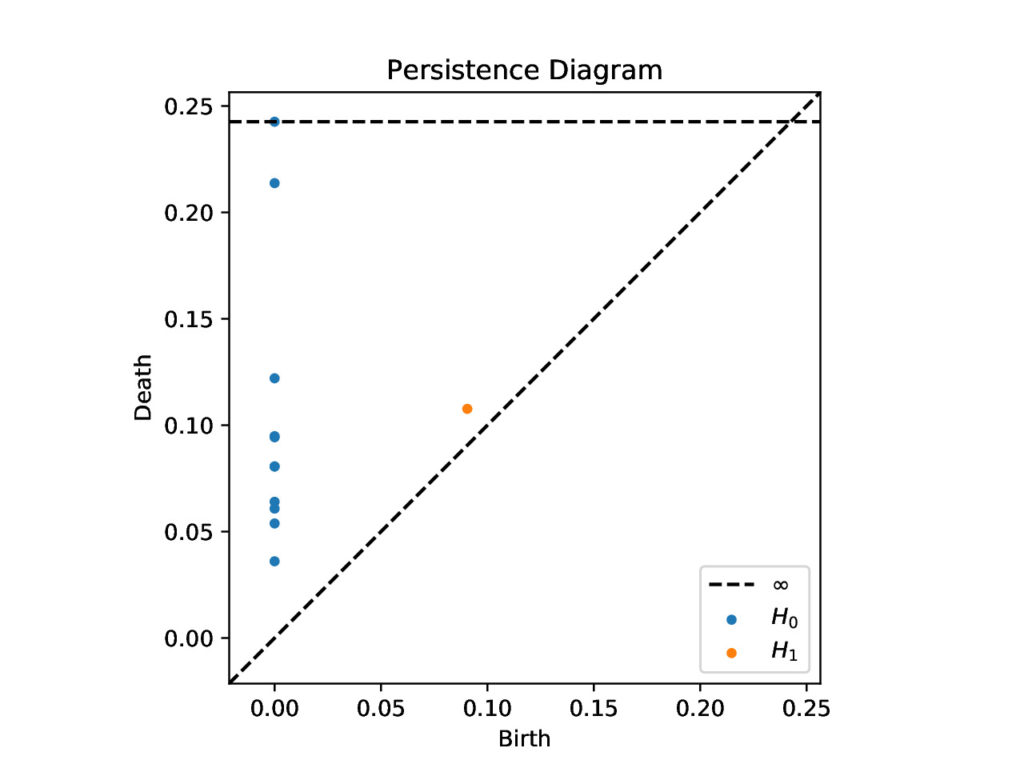
We represent the birth and death of each topological feature using persistence diagrams (the \(x\)-value of each point depicts when a feature was born and the \(y\)-values depicts when it died). For example, there is an orange dot at (birth, death) = (0.0905, 0.1077), because there is a loop born at \(\epsilon=0.0905\) that becomes filled in at \(\epsilon=0.1077\).
TDA and mathematical modeling
While we used TDA to summarize a simple collection of points in the
previous section, we can also use TDA to analyze complex patterns that
result from mathematical model simulations (Bhaskar et al., 2019).. Consider the agent-based model from D’Orsogna et al (2006): we have \(N\) interacting particles with two-dimensional positions, \(\mathbf{x}_i(t)=(x_i(t),y_i(t)), i=1,\dots,N\), and velocities, \(\mathbf{v}_i(t)=(v{x,i}(t),v_{y,i}(t))\), that change over time. Using Newton’s Law, we can determine a differential equation model for the motion of each particle’s position and velocity as follows:
The last equation above describes how forces of self propulsion (with parameter \(\alpha\)), friction (with parameter \(\beta\)), as well as attraction (with magnitude \(C_a\) over characteristic length \(\ell_a\)) and repulsion (with magnitude \(C_r\) over characteristic length \(\ell_r\)) between agents affect particle motion. When \(\alpha=1.5,\beta=0.5,C_a=1.0,C_r =0.1, \ell_a = 1.0, \ell_r= 0.1\), the model outputs a double ring pattern comprised of agents moving clockwise and counterclockwise (Fig. 6) (Bhaskar et al., 2019).

Persistent homology provides an informative way to summarize this observed patterning. We can create a four-dimensional point cloud comprised of the position and velocity information for each agent. We then compute the persistence diagram of the model snapshot from Figure 6 using this four dimensional data. We observe that two loops that are born near \(\epsilon=0.7\) and die near \(\epsilon=2.8\). These two loops likely correspond to the two rings moving clockwise or counter clockwise in the model simulation. Other model parameters will lead to different shapes and persistence diagrams; we encourage you to play around with the parameter values provided in Table 1 using the code provided at (Nardini, 2021)
| \(\alpha\) | \(\beta\) | \(C_\alpha\) | \(C_r\) | \(\ell_\alpha\) | \(\ell_r\) | |
| Parameter set 1 | 1.5 | 0.5 | 1.0 | 0.1 | 1.0 | 0.1 |
| Parameter set 2 | 1.5 | 0.5 | 1.0 | 0.5 | 1.0 | 0.1 |
| Parameter set 3 | 1.5 | 0.5 | 1.0 | 0.9 | 1.0 | 0.5 |
| Parameter set 4 | 1.5 | 0.5 | 1.0 | 0.1 | 1.0 | 0.5 |
| Parameter set 5 | 1.5 | 0.5 | 1.0 | 2.0 | 1.0 | 0.9 |
TDA computation
The python code used to generate the figures in this this tutorial is available at (Nardini, 2021). We use the Ripser python package to compute the persistent homology of the dataset because it has been found to be the best performing algorithm for computing the Vietoris-Rips complex (Otter et al. 2017; Traile et al. 2018). To understand to use linear algebra to compute the homology for a simplicial complex, we direct the interested reader to (Topaz, 2018).
References
Dhananjay Bhaskar, Angelika Manhart, Jesse Milzman, John T. Nardini, Kathleen M. Storey, Chad M. Topaz, Lori Ziegelmeier. Analyzing collective motion with machine learning and topology. Chaos, 29(12): 123125, 2019.@article{bhaskar2019analyzing,
title={Analyzing collective motion with machine learning and topology},
author={Bhaskar, Dhananjay and Manhart, Angelika and Milzman, Jesse and Nardini, John T. and Storey, Kathleen M. and Topaz, Chad M. and Ziegelmeier, Lori},
journal={Chaos},
year={2019},
number={12},
pages={123125},
publisher={American Institute of Physics}
}@article{d'orsogna2006self,
title={Self-Propelled Particles with Soft-Core Interactions: Patterns, Stability, and Collapse},
author={D'Orsogna, M. R. and Chuang, Y. L. and Bertozzi, A. L. and Chayes, L. S.},
journal={Phys. Rev. Lett.},
year={2006},
number={10},
pages={104302}
}@unpublished{john nardini2021tda_tutorial,
title={TDA\_tutorial},
author={John Nardini},
year={2021}
}@article{otter2017roadmap,
title={A roadmap for the computation of persistent homology},
author={Otter, Nina and Porter, Mason A. and Tillmann, Ulrike and Grindrod, Peter and Harrington, Heather A.},
journal={European Physical Journal -- Data Science},
year={2017},
number={17},
pages={1--38},
publisher={Springer}
}@unpublished{chad topaz2018chad's,
title={Chad's Self-Help Homology Tutorial for the Simple(x) Minded},
author={Chad Topaz},
year={2018}
}@article{christopher tralie 2018ripser.py,
title={Ripser.py: A Lean Persistent Homology Library for Python},
author={Christopher Tralie and Nathaniel Saul and Rann Bar-On},
journal={The Journal of Open Source Software},
year={2018},
pages={925},
publisher={The Open Journal}
}